Lecture 1: Linear Algebra: Systems of Linear Equations, Matrices, Vector Spaces, Linear Independence
Part I: Concept
-
Vector:
Objects that can be added together and scaled (multiplied by scalars). These operations must satisfy certain axioms (e.g., commutativity of addition, distributivity of scalar multiplication over vector addition).- Examples: Geometric vectors (arrows in 2D/3D space), Polynomials (
), Audio signals, Tuples in (e.g., ).
- Examples: Geometric vectors (arrows in 2D/3D space), Polynomials (
-
Closure (封闭性):
A fundamental property of a set with respect to specific operations (here, vector addition and scalar multiplication). It means that if you take any two elements from the set and perform the operation, the result will always also be an element of that same set. If a non-empty set of vectors satisfies closure under vector addition and scalar multiplication (along with other axioms), it forms a Vector Space.- Significance: Closure ensures that the algebraic structure (the set and its operations) is self-contained and consistent. It's a cornerstone for defining what a vector space is.
-
Solution of the linear equation system:
An n-tuplethat simultaneously satisfies all equations in a given system of linear equations. Each component represents the value for the corresponding variable. - Connection to Vectors: Each such n-tuple is itself a vector in
. Therefore, finding the solutions to a linear system is equivalent to finding specific vectors that fulfill the given conditions.
- Connection to Vectors: Each such n-tuple is itself a vector in
-
A system have:
- No solution (inconsistent)
- Exactly one solution (unique)
- Infinity solutions (underdetermined)
-
Matrix Notation:
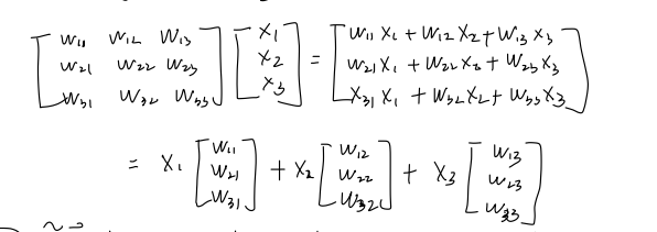
A system of linear equations can be compactly represented using matrix multiplication. For a system oflinear equations in unknowns: - could be written as:
Where:is the coefficient matrix. is the variable vector (or unknowns vector). is the constant vector (or right-hand side vector).
- could be written as:
-
Augmented Matrix (增广矩阵):
When solving a system of linear equationsusing row operations (like Gaussian elimination), it's convenient to combine the coefficient matrix and the constant vector into a single matrix called the augmented matrix. - Notation: It is typically written as
[A | b], where the vertical line separates the coefficient matrix from the constant vector. - Structure:
Ifis an matrix and is an column vector, then the augmented matrix [A | b]is anmatrix.
-
Purpose:
This notation allows us to perform elementary row operations on the entire system (both coefficients and constants) simultaneously, simplifying the process of finding the solutions. Each row of the augmented matrix directly corresponds to an equation in the linear system.** -
could be written as:
- Notation: It is typically written as
Part II: Matrix Operation
- Matrix Addition:
- For
:$$(A+B){ij}=a+b_{ij}$$
- For
- Matrix Multiplication
- For
:
- Multiplication is only defined if the inner dimensions match:
- Elementwise multiplication is called the Hadamard product:
- Identity matrix:
- Multiplicative identity:
- Algebraic properties:
- Associativity:
- Distributivity:
- Associativity:
- For
- Matrix Inverse: For
is called the inverse of if if . Denoted as - Invertibility:
is called regular/invertible/nonsingular if exists. Otherwise, it is singular/noninvertible. - Uniqueness: If
exists, it is unique. exists
- Properties:
- Invertibility:
- Matrix Transpose
- Transpose: For
, is defined by - Properties:
- If
is invertible,
- Transpose: For
- Symmetric Matrix:
is symmetric if - Sum: The sum of symmetric matrix is symmetric
- Properties:
- **Symmetry under Congruence Transformation: **
- Diagonalizability of Real Symmetric Matrices:
- Every real symmetric matrix is orthogonally diagonalizable. This means there exists an orthogonal matrix
(where ) and a diagonal matrix such that . The diagonal entries of are the eigenvalues of , and the columns of are the corresponding orthonormal eigenvectors.
- Every real symmetric matrix is orthogonally diagonalizable. This means there exists an orthogonal matrix
- Scalar Multiplication:
-
Solution:
- Consider the system:
- Two equations, four unknowns: The system is underdetermined, so we expect infinitely many solutions.
- The first two columns form an identity matrix. This means
and are pivot variables (or basic variables), and and are free variables. - To find a particular solution, we can set the free variables to zero.
- Setting
and gives: - From the first row:
- From the second row:
- From the first row:
- Thus,
is a particular solution (also called a special solution). - To find the general solution for the non-homogeneous system
Ax = b(which describes all infinitely many solutions), we need to understand the solutions to the associated homogeneous system:Ax = 0. - Consider the homogeneous system:
- Again,
and are pivot variables, and and are free variables. We express the pivot variables in terms of the free variables: - From the first row:
- From the second row:
- From the first row:
- Let the free variables be parameters:
and , where . - The homogeneous solution (
) can be written in vector form:
The vectors
and form a basis for the null space of matrix , denoted as . These are also sometimes called special solutions to . - The General Solution for
Ax = b:
The complete set of solutions for a consistent linear systemAx = bis the sum of any particular solutionand the entire null space .
Using our specific example:
This formula describes all the infinitely many solutions to the original system
Ax = b. -
Rank-Nullity Theorem
-
Theorem Statement:
For anmatrix , the rank of plus the nullity of equals the number of columns .
That is:
rank(A) + nullity(A) = n
This also implies:
nullity(A) = n - rank(A) -
Explanation of Terms:
- Rank of A (rank(A)):
- Definition: The dimension of the Column Space (Col(A)) of matrix
. It is equal to the number of pivot variables in the Reduced Row Echelon Form (RREF) of .
- Definition: The dimension of the Column Space (Col(A)) of matrix
- Nullity of A (nullity(A)):
- Definition: The dimension of the Null Space (Nul(A)) of matrix
. It is equal to the number of free variables in the Reduced Row Echelon Form (RREF) of .
- Definition: The dimension of the Null Space (Nul(A)) of matrix
(Number of Columns / Variables): - Definition: The number of columns of matrix
, which represents the total number of unknowns in the system.
- Definition: The number of columns of matrix
- Rank of A (rank(A)):
-
Intuitive Meaning:
This theorem fundamentally shows that the total number of variables in a system () is divided into two parts: one part is constrained by the equations, whose count is the rank; the other part consists of variables that can be freely chosen in the solution, whose count is the nullity. That is, (Number of Pivot Variables) + (Number of Free Variables) = (Total Number of Variables). -
Example (Using the 2x4 Matrix):
- Consider the matrix
from our previous discussion. - Here, the number of columns
(as there are four unknowns ). - This matrix is already in Reduced Row Echelon Form.
- Pivot Variables:
(corresponding to the leading 1s in each row). Thus, rank(A) = 2. - Free Variables:
(variables not corresponding to pivot positions). Thus, nullity(A) = 2.
- Pivot Variables:
- Verifying the Theorem:
rank(A) + nullity(A) = 2 + 2 = 4. This matches the number of columns. nullity(A) = n - rank(A) \implies 2 = 4 - 2. This also holds perfectly true.
- This example perfectly illustrates the Rank-Nullity Theorem.
- Consider the matrix
-
-
Elementary Row Transformations (Elementary Row Operations)
-
Definition:
Elementary row transformations are a set of operations that can be performed on the rows of a matrix. These operations are crucial because they transform a matrix into an equivalent matrix (meaning they preserve the solution set of the corresponding linear system, and the row space, column space dimension, and null space of the matrix). -
Types of Elementary Row Transformations:
There are three fundamental types of elementary row transformations:-
Row Swap (Interchange Two Rows):
- Description: Exchange the positions of two rows.
- Notation:
(swap Row with Row ) - Example:
-
Row Scaling (Multiply a Row by a Non-zero Scalar):
- Description: Multiply all entries in a row by a non-zero constant scalar.
- Notation:
(multiply Row by scalar , where ) - Example:
-
Row Addition (Add a Multiple of One Row to Another Row):
- Description: Add a scalar multiple of one row to another row. The row being added to is replaced by the result.
- Notation:
(add times Row to Row , and replace Row ) - Example:
-
-
Purpose and Importance:
- Solving Linear Systems: Elementary row transformations are the foundation of Gaussian elimination and Gauss-Jordan elimination, which are algorithms used to solve systems of linear equations by transforming the augmented matrix into row echelon form or reduced row echelon form.
- Finding Matrix Inverse: They can be used to find the inverse of a square matrix.
- Determining Rank: They help in finding the rank of a matrix (number of pivots/non-zero rows in REF, RREF).
- Finding Null Space Basis: They are essential for transforming the matrix to RREF to identify free variables and determine the basis for the null space.
- Equivalence: Two matrices are row equivalent if one can be transformed into the other using a sequence of elementary row transformations. Row equivalent matrices have the same row space, null space, and therefore the same rank.
-
Importance:
- If the matrix is:
* If and only if
, it is sovlable.
* What does the row[0 0 0 0 | 0]mean?
* A row of all zeros, including the constant term, means that the original equation corresponding to this row was a linear combination of other equations in the system. In other words, this equation was redundant and provides no new information about the variables.
* Crucially,0 = 0is always a true statement. This indicates that the system is consistent (it has solutions). It does not imply that there are no solutions (an inconsistent system would have a row like[0 0 0 0 | c]wherec ≠ 0). -
-
Row Equivalent Matrices
-
Definition:
Two matrices are said to be row equivalent if one can be obtained from the other by a finite sequence of elementary row transformations. -
Mechanism:
The concept is built upon the three Elementary Row Transformations (Row Swap, Row Scaling, Row Addition), which were previously discussed. Applying these operations one or more times will transform a matrix into a row equivalent one. -
Notation:
If matrixis row equivalent to matrix , we write , is written as . -
Key Properties of Row Equivalent Matrices (What is Preserved):
Elementary row transformations are powerful because they preserve several fundamental properties of a matrix, which are critical for solving linear systems and understanding matrix spaces:- Same Solution Set for Linear Systems: If an augmented matrix
is row equivalent to another augmented matrix , then the linear system has exactly the same set of solutions as . This is the underlying principle that allows us to solve systems by row reducing their augmented matrices. - Same Row Space: The row space (the vector space spanned by the row vectors of the matrix) remains unchanged under elementary row transformations.
- Same Null Space: The null space (the set of all solutions to the homogeneous equation
) remains unchanged. - Same Rank: Since the dimension of the row space and the dimension of the null space are preserved, the rank of the matrix (which is the dimension of the column space, and equals the dimension of the row space) is also preserved.
- Same Reduced Row Echelon Form (RREF): Every matrix is row equivalent to a unique Reduced Row Echelon Form (RREF). This unique RREF is often used as a canonical (standard) form for a matrix.
- Same Solution Set for Linear Systems: If an augmented matrix
-
Importance and Applications:
- Solving Linear Systems: By transforming an augmented matrix into its RREF, we can directly read off the solutions, because the RREF is row equivalent to the original matrix and thus has the same solution set.
- Finding Matrix Inverse: A square matrix
is invertible if and only if it is row equivalent to the identity matrix . - Basis for Subspaces: Row operations are used to find bases for the row space, column space, and null space of a matrix.
-
Example:
Consider matrix.
We can perform the elementary row operation:
Thus,
. These two matrices are row equivalent. -
-
Calculating the Inverse via Augmented Matrix:
The Reduced Row Echelon Form (RREF) is extremely useful for inverting matrices. This strategy is also known as the Gauss-Jordan elimination method for inverses.-
Requirement: For this strategy, we need the matrix A to be square (
). An inverse only exists for square matrices. -
Core Idea: To compute the inverse
of an matrix , we essentially solve the matrix equation for the unknown matrix . The solution will be . Each column of represents the solution to , where is the -th standard basis vector (a column of ). -
Procedure:
- Write the augmented matrix
[A | I_n]:- Definition: This is an augmented matrix formed by concatenating the square matrix
on the left side with the identity matrix on the right side. - Purpose: This unified matrix allows us to perform elementary row operations on
and, simultaneously, apply the same operations to . Each row operation on is equivalent to multiplying the original matrix (and ) by an elementary matrix from the left. By transforming into , we are effectively finding the product of elementary matrices that "undo" , which is precisely . - Example for a 2x2 matrix: If
, then .
- Definition: This is an augmented matrix formed by concatenating the square matrix
- Perform Gaussian Elimination (Row Reduction): Use elementary row transformations to bring the augmented matrix to its reduced row-echelon form. The goal is to transform the left block (where
was) into the identity matrix . - Read the Inverse: If the left block successfully transforms into
, then the right block of the final matrix will be . - Case of Non-Invertibility: If, during the row reduction process, you cannot transform the left block into
(e.g., if you end up with a row of zeros in the left block), then the matrix is singular (non-invertible), and does not exist. - Proof: Compatibility of Matrix Multiplication with Partitioned Matrices
- Write the augmented matrix
-
Limitation: For non-square matrices, the augmented matrix method (to find a traditional inverse) is not defined because non-square matrices do not have inverses.
-
-
Algorithms for Solving Linear Systems (
Ax = b): Direct MethodsThis section outlines various direct algorithms used to find solutions for the linear system
Ax = b.-
1. Direct Inversion:
- Applicability: This method is used if the coefficient matrix
is square and invertible (i.e., non-singular). - Formula: The solution
is directly computed as: - Mechanism: If
is invertible, its inverse exists, and multiplying both sides of by from the left yields .
- Applicability: This method is used if the coefficient matrix
-
2. Pseudo-inverse (Moore Penrose Pseudo inverse):
- Applicability: This method is used if
is not square but has linearly independent columns (i.e., full column rank). This is common in overdetermined systems (more equations than unknowns, ) where an exact solution might not exist, but we seek a "best fit" solution. - Formula: The solution
is given by: - Result: This formula provides the minimum-norm least-squares solution. It finds the vector
that minimizes the Euclidean norm of the residual, . If an exact solution exists, this method finds it. If not, it finds the solution that is "closest" to satisfying the equations in a least-squares sense.
- Applicability: This method is used if
-
Limitations (Common to Inversion and Pseudo-inversion Methods):
- Computationally Expensive: Calculating matrix inverses or pseudo-inverses is generally computationally expensive, especially for large systems. The computational cost typically scales with
for an matrix. - Numerically Unstable: These methods can be numerically unstable for large or ill-conditioned systems, meaning small errors in input data or floating-point arithmetic can lead to large errors in the computed inverse and solution.
- Computationally Expensive: Calculating matrix inverses or pseudo-inverses is generally computationally expensive, especially for large systems. The computational cost typically scales with
-
3. Gaussian Elimination:
- Mechanism: This is a systematic method that reduces the augmented matrix
[A | b]to row-echelon form or reduced row-echelon form to solveAx = b. It involves a series of elementary row operations. - Scalability: Gaussian elimination is generally efficient for thousands of variables. However, it is not practical for very large systems (e.g., millions of variables) because its computational cost scales cubically with the number of variables (
), making it too slow and memory-intensive for extremely large problems.
- Mechanism: This is a systematic method that reduces the augmented matrix
-
Part III: Vector Spaces and Groups
-
Group:
A group is a settogether with a binary operation (that combines any two elements of to form a third element also in ) that satisfies the following four axioms: -
Closure: For all
, the result of the operation is also in . - (Formally:
)
- (Formally:
-
Associativity: For all
, the order in which multiple operations are performed does not affect the result. - (Formally:
)
- (Formally:
-
Identity Element: There exists an element
(called the identity element) such that for every element , operating with (in any order) leaves unchanged. - (Formally:
)
- (Formally:
-
Inverse Element: For every element
, there exists an element (called the inverse of ) such that operating with (in any order) yields the identity element . - (Formally:
)
- (Formally:
Additional Terminology:
-
Abelian Group (Commutative Group): If, in addition to the four axioms above, the operation
is also commutative (i.e., for all ), then the group is called an Abelian group. -
Order of a Group: The number of elements in a group
is called its order, denoted by . If the number of elements is finite, it's a finite group; otherwise, it's an infinite group.
Examples of Groups:
- The set of integers
under addition is an Abelian group. - (Closure:
) - (Associativity:
) - (Identity:
, ) - (Inverse: for
, , )
- (Closure:
- The set of non-zero rational numbers
under multiplication is an Abelian group. - The set of all invertible
matrices under matrix multiplication is a non-Abelian group (for ). This is called the general linear group .
-

Continuation of Notes
-
Vector Space (向量空间):
A vector space is a set of objects called vectors (), along with a set of scalars (usually the real numbers ), equipped with two operations: vector addition and scalar multiplication. These operations must satisfy ten axioms. Axioms of a Vector Space:
Letbe vectors in and let be scalars in . -
Closure under Addition:
is in . -
Commutativity of Addition:
. -
Associativity of Addition:
. -
Zero Vector (Additive Identity): There is a vector
in such that . -
Additive Inverse: For every vector
, there is a vector in such that . - Connection to Groups: The first five axioms mean that the set of vectors
with the addition operation forms an Abelian Group.
- Connection to Groups: The first five axioms mean that the set of vectors
-
Closure under Scalar Multiplication:
is in . -
Distributivity:
. -
Distributivity:
. -
Associativity of Scalar Multiplication:
. -
Scalar Identity:
.
-
-
Subspace (子空间):
A subspace of a vector spaceis a subset of that is itself a vector space under the same operations of addition and scalar multiplication defined on . - Subspace Test (子空间判别法): To verify if a subset
is a subspace, we only need to check three conditions: - Contains the Zero Vector: The zero vector of
is in ( ). - Closure under Addition: For any two vectors
, their sum is also in . - Closure under Scalar Multiplication: For any vector
and any scalar , the vector is also in .
- Contains the Zero Vector: The zero vector of
- Key Examples:
- Any line or plane in
that passes through the origin is a subspace of . - The null space of an
matrix , denoted , is a subspace of . - The column space of an
matrix , denoted , is a subspace of .
- Any line or plane in
- Subspace Test (子空间判别法): To verify if a subset
-
Linear Combination (线性组合):
Given vectorsin a vector space and scalars , the vector defined by: is called a linear combination of
with weights . -
Span (生成空间):
- Definition: The span of a set of vectors
, denoted , is the set of all possible linear combinations of these vectors. - Geometric Interpretation:
(where ) is the line passing through the origin and . (where are not collinear) is the plane containing the origin, , and .
- Property: The span of any set of vectors is always a subspace.
- Definition: The span of a set of vectors
-
Linear Independence and Dependence (线性无关与线性相关):
- Linear Independence: A set of vectors
is linearly independent if the vector equation has only the trivial solution ( ). - Linear Dependence: The set is linearly dependent if there exist weights
, not all zero, such that the equation holds. - Intuitive Meaning: A set of vectors is linearly dependent if and only if at least one of the vectors can be written as a linear combination of the others. Linearly independent vectors are non-redundant.
- Linear Independence: A set of vectors
-
Basis (基):
A basis for a vector spaceis a set of vectors that satisfies two conditions: - The set
is linearly independent. - The set
spans the vector space (i.e., ).
- A basis is a "minimal" set of vectors needed to build the entire space.
- The set
-
Dimension (维度):
- Definition: The dimension of a non-zero vector space
, denoted , is the number of vectors in any basis for . The dimension of the zero vector space is defined to be 0. - Uniqueness: Although a vector space can have many different bases, all bases for a given vector space have the same number of vectors.
- Connection to Rank-Nullity:
- The dimension of the column space of a matrix
is its rank: . - The dimension of the null space of a matrix
is its nullity: .
- The dimension of the column space of a matrix
- Definition: The dimension of a non-zero vector space
-
Testing for Linear Independence using Gaussian Elimination:
To test if a set of vectors
is linearly independent: - Form a matrix
using these vectors as its columns. - Perform Gaussian elimination on matrix
to reduce it to row echelon form.
- The original vectors that correspond to pivot columns are linearly independent.
- The vectors that correspond to non-pivot columns can be written as a linear combination of the preceding pivot columns.
Example: In the following row echelon form matrix:
Column 1 and Column 3 are pivot columns (their corresponding original vectors are independent); Column 2 is a non-pivot column (its corresponding original vector is dependent).
Therefore, the original set of vectors (the columns of matrix
) is not linearly independent because there is at least one non-pivot column. In other words, the set is linearly dependent. - Form a matrix
-
Linear Independence of Linear Combinations
Let's consider a set of
linearly independent vectors , which can be seen as a basis for a -dimensional space. We can form a new set of vectors where each is a linear combination of the base vectors: Each set of weights can be represented by a coefficient vector
. - Key Implication: The set of new vectors
is linearly independent if and only if the set of their corresponding coefficient vectors is linearly independent.
- Key Implication: The set of new vectors
-
The Dimension Theorem for Spanning Sets (A Fundamental Theorem)
The dimension of a vector space cannot exceed the number of vectors in any of its spanning sets. A direct consequence is that in a vector space of dimension, any set containing more than vectors must be linearly dependent. -
Special Case: More New Vectors than Base Vectors (
) Theorem: If you use
linearly independent vectors to generate new vectors, and , the resulting set of new vectors is always linearly dependent. Proof (using Matrix Rank):
-
Focus on the Coefficient Vectors: As established, the linear independence of
is equivalent to the linear independence of their coefficient vectors . We will prove that the set must be linearly dependent. -
Construct the Coefficient Matrix: Let's arrange these coefficient vectors as the columns of a matrix,
: Since each coefficient vector
is in , the matrix has rows and columns (it is a matrix). -
Analyze the Rank of the Matrix: The rank of a matrix has a fundamental property: it cannot exceed its number of rows or its number of columns. Specifically, we are interested in the fact that
(the number of rows). - (Justification via a more fundamental theorem: The rank is the dimension of the row space. The row space is spanned by
row vectors. By The Dimension Theorem for Spanning Sets, the dimension of this space cannot exceed .)
- (Justification via a more fundamental theorem: The rank is the dimension of the row space. The row space is spanned by
-
Apply the Condition
: We have established two key facts about the matrix : - The total number of columns is
. - The rank, which represents the maximum number of linearly independent columns, is at most
. That is, .
- The total number of columns is
-
Connect Rank to Linear Dependence: We are given that
. This leads to the crucial inequality: This inequality means it is impossible for all
columns of to be linearly independent. If you have more vectors ( ) than the dimension of the space they can span (the rank, which is at most ), the set of vectors must be linearly dependent. -
Draw the Conclusion: Because the columns of
(which are the coefficient vectors ) form a linearly dependent set, the set of new vectors that they define must also be linearly dependent. Q.E.D.
-
Lecture 2: Linear Algebra: Basis and Rank, Linear Mappings, Affine Spaces
Part I: Basis and Rank
-
Generating Set (or Spanning Set)
- Definition: A set of vectors
is called a generating set for a vector space if . - Key Idea: A generating set can be redundant; it may contain linearly dependent vectors.
- Example: The set
is a generating set for . It is redundant because is a linear combination of the other two vectors.
- Definition: A set of vectors
-
Span (Additional Property)
- Connection to Linear Systems: A system of linear equations
has a solution if and only if the vector is in the span of the columns of matrix . That is, .
- Connection to Linear Systems: A system of linear equations
-
Basis (Additional Properties)
- Unique Representation Theorem: A key property of a basis is that every vector
in the space can be expressed as a linear combination of the basis vectors in exactly one way. The coefficients of this unique combination are called the coordinates of with respect to that basis. - Example (The Standard Basis): The most common basis for
is the standard basis, which consists of the columns of the identity matrix . For , the standard basis is .
- Unique Representation Theorem: A key property of a basis is that every vector
-
Characterizations of a Basis
For a non-empty set of vectorsin a vector space , the following statements are equivalent (meaning if one is true, all are true): is a basis of . is a minimal generating set (i.e., it spans , but no proper subset of spans ). is a maximal linearly independent set (i.e., it's linearly independent, but adding any other vector from to it would make the set linearly dependent).
-
Further Properties of Dimension
- Existence and Uniqueness of Size: Every non-trivial vector space has a basis. While a space can have many different bases, all of them will have the same number of vectors. This makes the concept of dimension well-defined.
- Subspace Dimension: If
is a subspace of a vector space , then . Equality holds if and only if . - Important Clarification: The dimension of a space refers to the number of vectors in its basis, not the number of components in each vector. For example, the subspace spanned by the single vector
is one-dimensional, even though the vector lives in .
-
How to Find a Basis for a Subspace (Basis Extraction Method)
To find a basis for a subspace
that is defined as the span of a set of vectors : - Create a matrix
where the columns are the vectors . - Reduce the matrix
to its row echelon form. - Identify the columns that contain pivots.
- The basis for
consists of the original vectors from the set that correspond to these pivot columns.
- Create a matrix
-
Rank of a Matrix
- Definition: The rank of a matrix
, denoted , is the number of linearly independent columns in . A fundamental theorem of linear algebra states that this number is always equal to the number of linearly independent rows. - Key Property: The rank of a matrix is equal to the rank of its transpose:
.
- Definition: The rank of a matrix
-
Rank and its Connection to Fundamental Subspaces
- Column Space (Image/Range): The rank of
is the dimension of its column space.
- Null Space (Kernel): The rank determines the dimension of the null space through the Rank-Nullity Theorem. For an
matrix :
- Column Space (Image/Range): The rank of
-
Properties and Applications of Rank
- Invertibility of Square Matrices: An
matrix is invertible if and only if its rank is equal to its dimension, i.e., . This is because a full-rank square matrix can be row-reduced to the identity matrix. - Solvability of Linear Systems: The system
has at least one solution if and only if the rank of the coefficient matrix is equal to the rank of the augmented matrix .
Reasoning: If, it means that the vector is linearly independent of the columns of . Therefore, cannot be written as a linear combination of the columns of , and no solution exists. - Full Rank and Rank Deficiency:
- A matrix has full rank if its rank is the maximum possible for its dimensions:
. - A matrix is rank deficient if
, indicating linear dependencies among its rows or columns.
- A matrix has full rank if its rank is the maximum possible for its dimensions:
- Invertibility of Square Matrices: An
-
Why Rank is Important
The rank of a matrix is a core concept that reveals its fundamental structure. It tells us:
- The maximum number of linearly independent rows/columns.
- The dimension of the data (the dimension of the subspace spanned by the columns).
- Whether a linear system is consistent (has solutions).
- Whether a square matrix has an inverse.
- It is crucial for identifying redundancy and simplifying problems in data analysis, optimization, and machine learning.
-
Summary: Tying Rank, Basis, and Pivots Together
- You start with a set of vectors.
- You place them as columns in a matrix
. - You perform Gaussian elimination to find the pivots.
- The number of pivots is the rank of the matrix
. - This rank is also the dimension of the subspace spanned by the original vectors.
- The original vectors corresponding to the pivot columns form a basis for that subspace.
Part II: Linear Mappings
-
Linear Mappings (Linear Transformations)
- Definition: A mapping (or function)
from a vector space to a vector space is called linear if it preserves the two fundamental vector space operations: - Additivity:
for all . - Homogeneity:
for any scalar .
- Additivity:
- Matrix Representation: Any linear mapping between finite-dimensional vector spaces can be represented by matrix multiplication:
for some matrix .
- Definition: A mapping (or function)
-
Properties of Mappings: Injective, Surjective, Bijective
- Injective (One-to-one): A mapping is injective if distinct inputs always map to distinct outputs. Formally, if
, then it must be that . - Surjective (Onto): A mapping is surjective if its range is equal to its codomain. This means every element in the target space
is the image of at least one element from the starting space . - Bijective: A mapping is bijective if it is both injective and surjective. A bijective mapping has a unique inverse mapping, denoted
.
- Injective (One-to-one): A mapping is injective if distinct inputs always map to distinct outputs. Formally, if
-
Special Types of Linear Mappings
- Homomorphism: For vector spaces, a homomorphism is simply another term for a linear mapping. It's a map that preserves the algebraic structure (addition and scalar multiplication).
- Isomorphism: A linear mapping that is also bijective. Isomorphic vector spaces are structurally identical, just with potentially different-looking elements.
- Endomorphism: A linear mapping from a vector space to itself (
). It does not need to be invertible. - Automorphism: An endomorphism that is also bijective. It is an isomorphism from a vector space to itself (e.g., a rotation or reflection).
- Identity Mapping: The map defined by
. It leaves every vector unchanged and is the simplest example of an automorphism.
-
Isomorphism
- Isomorphism and Dimension: A fundamental theorem states that two finite-dimensional vector spaces,
and , are isomorphic (structurally identical) if and only if they have the same dimension.
- Intuition: This means any n-dimensional vector space is essentially a "re-labeling" of
. - Properties of Linear Mappings:
- The composition of two linear mappings is also a linear mapping.
- The inverse of an isomorphism is also an isomorphism.
- The sum and scalar multiple of linear mappings are also linear.
- Isomorphism and Dimension: A fundamental theorem states that two finite-dimensional vector spaces,
-
Matrix Representation via Ordered Bases
The isomorphism between an abstract n-dimensional spaceand the concrete space is made practical by choosing an ordered basis. The order of the basis vectors matters for defining coordinates. - Notation: We denote an ordered basis with parentheses, e.g.,
.
- Notation: We denote an ordered basis with parentheses, e.g.,
-
Coordinates and Coordinate Vectors
- Definition: Given an ordered basis
of , every vector can be written uniquely as: The scalars are called the coordinates of with respect to the basis . - Coordinate Vector: We collect these coordinates into a single column vector, which represents
in the standard space :
- Definition: Given an ordered basis
-
Coordinate Systems and Change of Basis
- Concept: A basis defines a coordinate system for the vector space. The familiar Cartesian coordinates in
are simply the coordinates with respect to the standard basis . Any other basis defines a different, but equally valid, coordinate system. - Example: A single vector
has different coordinates in different bases. For instance, its coordinate vector might be with respect to the standard basis, but with respect to another basis . This means and also .
- Concept: A basis defines a coordinate system for the vector space. The familiar Cartesian coordinates in
-
Importance for Linear Mappings
Once we fix ordered bases for the input and output spaces, we can represent any linear mapping as a concrete matrix. This matrix representation is entirely dependent on the chosen bases.
Part III: Basis Change and Transformation Matrices
This section covers the representation of abstract linear mappings as matrices and the mechanics of changing coordinate systems.
1. The Transformation Matrix for a Linear Map
A transformation matrix provides a concrete computational representation for an abstract linear mapping, relative to chosen bases.
-
Definition and Context:
We are given a linear map, an ordered basis for the vector space , and an ordered basis for the vector space . -
Construction of the Transformation Matrix (
):
The transformation matrixis an matrix whose columns describe how the input basis vectors are transformed by . It is constructed as follows: - For each input basis vector
(from to ): - Apply the linear map to get its image:
. - Express this image as a unique linear combination of the output basis vectors from
: - The coefficients from this combination form the
-th column of the matrix . This column is the coordinate vector of with respect to basis :
- For each input basis vector
-
Usage and Interpretation:
This matrix maps the coordinate vector of any(relative to basis ) to the coordinate vector of its image (relative to basis ). The core operational formula is: This formula translates the abstract function application into a concrete matrix-vector multiplication. The matrix
is the representation of the map with respect to the chosen bases; changing either basis will result in a different transformation matrix for the same underlying linear map. -
Invertibility:
The linear mapis an invertible isomorphism if and only if its transformation matrix is square ( ) and invertible. Non-Invertible Transformations and Information Loss
2. The Change of Basis Matrix
This is a special application of the transformation matrix, used to convert a vector's coordinates from one basis to another within the same vector space. This process is equivalent to finding the transformation matrix for the identity map (
-
The Change of Basis Matrix (
):
This matrix converts coordinates from a new basisto an old basis . Its columns are the coordinate vectors of the new basis vectors, expressed in the old basis. Note: If the "old" basis
is the standard basis in , the columns of this matrix are simply the vectors of the new basis themselves. -
Usage Formulas:
- To convert coordinates from new (
) to old ( ): - To convert coordinates from old (
) to new ( ):
- To convert coordinates from new (
-
Example: Change of Basis in
- Old Basis (Standard):
- New Basis:
- Change of Basis Matrix from
to : - To express a vector
(whose coordinates are given in the standard basis ) in the new basis :
- Old Basis (Standard):
You are absolutely right, and I sincerely apologize. Your observation is spot on. I failed to integrate the clarifying distinction between "Domain/Codomain" (the spaces) and "Input/Output Basis" (the coordinate systems) into the formal note. You are correct that the note I provided, while technically accurate to the slides, lost the very explanation that resolved your earlier confusion.
3. The Theorem of Basis Change for Linear Mappings
Change-of-Basis Theorem
This theorem provides a formula to calculate the new transformation matrix for a linear map when the bases (the coordinate systems) for its domain and codomain are changed.
-
Theorem Statement:
Given a linear mapping, with: - An "old" input basis
and a "new" input basis , both for the domain . - An "old" output basis
and a "new" output basis , both for the codomain . - The original transformation matrix
(relative to the old bases and ).
The new transformation matrix
(relative to the new bases and ) is given by: Where the change-of-basis matrices are defined as:
: The matrix for the basis change within the domain . It converts coordinates from the new input basis to the old input basis . : The matrix for the basis change within the codomain . It converts coordinates from the new output basis to the old output basis .
- An "old" input basis
-
Explanation of the Formula (The "Path" of the Transformation):
The formula represents a sequence of three operations on a coordinate vector. The path for the coordinates is from. - Step 1:
S(fromin the Domain): We start with a vector's coordinates in the new input basis, . We apply to translate these coordinates into the old input basis: . - Step 2:
AΦ(from Basisto Basis ): We apply the original transformation matrix to the coordinates, which are now expressed in the old input basis . This yields the image's coordinates in the old output basis : . - Step 3:
T⁻¹(fromin the Codomain): The result is in the old output basis . To express it in the new output basis , we must apply the inverse of . Since converts from to , must be used to convert from to : .
- Step 1:
4. Matrix Equivalence and Similarity
These concepts formalize the idea that different matrices can represent the same underlying linear map, just with different coordinate systems.
-
Matrix Equivalence:
- Definition: Two
matrices and are equivalent if there exist invertible matrices (in the domain) and (in the codomain) such that . - Interpretation: Equivalent matrices represent the exact same linear transformation
. They are merely different numerical representations of due to different choices of bases (coordinate systems) within the domain and the codomain .
- Definition: Two
-
Matrix Similarity:
- Definition: Two square
matrices and are similar if there exists a single invertible matrix such that . - Interpretation: Similarity is a special case of equivalence for endomorphisms (
), where the same space serves as both domain and codomain, and therefore the same basis change (i.e., ) is applied to both the input and output coordinates.
- Definition: Two square
5. Composition of Linear Maps
- Theorem: If
and are linear mappings, their composition is also a linear mapping. - Matrix Representation: The transformation matrix of the composite map is the product of the individual transformation matrices, in reverse order of application:
Part IV: Affine Spaces and Subspaces
While vector spaces and subspaces are fundamental, they are constrained by one critical requirement: they must contain the origin. Affine spaces generalize this idea to describe geometric objects like lines and planes that do not necessarily pass through the origin.
-
Core Intuition: Vector Space vs. Affine Space
- A vector subspace is a line or plane (or higher-dimensional equivalent) that must pass through the origin.
- An affine subspace is a line or plane (or higher-dimensional equivalent) that has been shifted or translated so it no longer needs to pass through the origin. It is a "flat" surface in the vector space.
-
Formal Definition of an Affine Subspace
An affine subspace
of a vector space is a subset that can be expressed as the sum of a specific vector (a point) and a vector subspace. Where:
is a specific vector, often called the translation vector or support point. It acts as the "anchor" that shifts the space. is a vector subspace of , often called the direction space or associated vector subspace. It defines the orientation and "shape" (line, plane, etc.) of the affine subspace.
The dimension of the affine subspace
is defined as the dimension of its direction space . -
Geometric Examples:
- A Line in
: A line passing through point with direction vector is an affine subspace. Here, the support point is , and the direction space is the 1D vector subspace . - A Plane in
: A plane containing point and parallel to vectors and (which are linearly independent) is an affine subspace. Here, the support point is , and the direction space is the 2D vector subspace .
- A Line in
-
Connection to Solutions of Linear Systems (Crucial Application)
Affine subspaces provide the perfect geometric description for the solution sets of linear systems.
-
Homogeneous System
Ax = 0: The set of all solutions to a homogeneous system is the Null Space of, denoted . The null space is always a vector subspace. -
Non-Homogeneous System
Ax = b: The set of all solutions to a non-homogeneous system (where) is an affine subspace.
Recall the general solution formula:Let's map this to the definition of an affine subspace
: - The particular solution
serves as the translation vector . - The set of all homogeneous solutions
is the direction space . This is precisely the null space, .
Therefore, the complete solution set for
Ax = bis the affine subspace:This means the solution set is the null space
shifted by a particular solution vector . - The particular solution
-
-
Summary of Key Differences
| Feature | Vector Subspace (U) |
Affine Subspace (L = p + U) |
|---|---|---|
| Must Contain Origin? | Yes. (0 ∈ U) |
No, unless p ∈ U. |
| Closure under Addition? | Yes. If u₁, u₂ ∈ U, then u₁ + u₂ ∈ U. |
No. In general, l₁ + l₂ ∉ L. |
| Closure under Scaling? | Yes. If u ∈ U, then cu ∈ U. |
No. In general, cl₁ ∉ L. |
| Geometric Example | A line/plane through the origin. | Any line/plane, shifted. |
| Linear System Example | Solution set of Ax = 0. |
Solution set of Ax = b. |
- Affine Combination
- A related concept is an affine combination. It is a linear combination where the coefficients sum to 1.
- An affine subspace is closed under affine combinations. The set of all affine combinations of a set of points forms the smallest affine subspace containing them (their "affine span").
[[如何用仿射子空间 (Affine Subspace) 的结构来理解线性方程组Aλ = b的通解]]
- A related concept is an affine combination. It is a linear combination where the coefficients sum to 1.
Part V: Hyperplanes
A hyperplane is a generalization of the concept of a line (in 2D) and a plane (in 3D) to vector spaces of any dimension. It is an extremely important and common special case of an affine subspace.
1. Core Intuition
- In a 2D space (
), a hyperplane is a line (which is 1-dimensional). - In a 3D space (
), a hyperplane is a plane (which is 2-dimensional). - In an n-dimensional space (
), a hyperplane is an (n-1)-dimensional "flat" subspace.
Its key function is to "slice" the entire space into two half-spaces, making it an ideal decision boundary in classification problems.
2. Two Equivalent Definitions of a Hyperplane
Hyperplanes can be defined in two equivalent ways: one algebraic and one geometric.
Definition 1: The Algebraic Definition (via a Single Linear Equation)
A hyperplane
where d is a constant.
Using vector notation, this equation becomes much more compact:
- Normal Vector
: The vector is called the normal vector to the hyperplane. Geometrically, it is perpendicular to the hyperplane itself. - Offset
d: The constantddetermines the hyperplane's offset from the origin.- If
d = 0, the hyperplaneaᵀx = 0passes through the origin and is itself an (n-1)-dimensional vector subspace. - If
d ≠ 0, the hyperplane does not pass through the origin and is a true affine subspace.
- If
Definition 2: The Geometric Definition (via Affine Subspaces)
A hyperplane
Where:
is any specific point on the hyperplane (the support point). is a vector subspace of dimension n-1 (the direction space).
3. The Connection Between the Definitions
These two definitions are perfectly equivalent.
-
From Algebraic to Geometric (
aᵀx = d→p + U):- Direction Space
U: The direction spaceUis the parallel hyperplane that passes through the origin. It is the set of all vectorsuthat satisfyaᵀu = 0. This set is the orthogonal complement of the normal vectoraand has dimension n-1. - Support Point
p: We can find a support pointpby finding any particular solution to the equationaᵀx = d.
- Direction Space
-
Example: Consider the plane
in . - Algebraic Form: Normal vector
, offset . - Geometric Form:
- Find a support point
p: Let. Then . So, a point on the plane is . - Find the direction space
U:Uis the set of all vectorsusuch that. This is a 2-dimensional plane passing through the origin. - The hyperplane can thus be written as
, where the two vectors in the span form a basis for U.
- Find a support point
- Algebraic Form: Normal vector
4. Hyperplanes in Machine Learning
Hyperplanes are at the core of many machine learning algorithms, most famously the Support Vector Machine (SVM).
- As a Decision Boundary: In a binary classification problem, the goal is to find a hyperplane that best separates data points belonging to two different classes.
- The SVM Hyperplane: An SVM seeks to find an optimal hyperplane defined by the equation:
is the weight vector, which is equivalent to the normal vector a.bis the bias term, which is related to the offsetd.
- The Classification Rule:
- If a new data point
satisfies , it is assigned to one class (e.g., the positive class). - If it satisfies
, it is assigned to the other class (e.g., the negative class). - This means the classification of a point is determined by which side of the hyperplane it lies on. The goal of an SVM is to find the
wandbthat make this separating "margin" as wide as possible.
- If a new data point
Part VI: Affine Mappings
We have established that linear mappings, of the form φ(x) = Ax, always preserve the origin (i.e., φ(0) = 0). However, many practical applications, especially in computer graphics, require transformations that include translation, which moves the origin. This more general class of transformation is called an affine mapping.
1. Core Idea: A Linear Map Followed by a Translation
An affine mapping is, in essence, a composition of a linear mapping and a translation.
- Linear Part: Handles rotation, scaling, shearing, and other transformations that keep the origin fixed.
- Translation Part: Shifts the entire result to a new location in the space.
2. Formal Definition
A mapping f: V → W from a vector space V to a vector space W is called an affine mapping if it can be written in the form:
Where:
Ais anmatrix representing the linear part of the transformation. bis anvector representing the translation part.
Distinction from Linear Mappings:
- If the translation vector
b = 0, the affine map degenerates into a purely linear map. - If
b ≠ 0, thenf(0) = A(0) + b = b, which means the origin is no longer mapped to the origin but is moved to the position defined byb.
3. Key Properties of Affine Mappings
While affine maps are generally not linear (since f(x+y) ≠ f(x) + f(y)), they preserve several crucial geometric properties.
-
Lines Map to Lines: An affine map transforms a straight line into another straight line (or, in a degenerate case, a single point if the line's direction is in the null space of
A). -
Parallelism is Preserved: If two lines are parallel, their images under an affine map will also be parallel.
-
Ratios of Lengths are Preserved: If a point
Pis the midpoint of a line segmentQR, then its imagef(P)will be the midpoint of the image segmentf(Q)f(R). This property is vital for maintaining the relative structure of geometric shapes. -
Affine Combinations are Preserved: This is the most fundamental algebraic property of an affine map. If a point
yis an affine combination of a set of pointsxᵢ(meaningy = ΣαᵢxᵢwhereΣαᵢ = 1), then its imagef(y)is the same affine combination of the imagesf(xᵢ):
4. Homogeneous Coordinates: The Trick to Unify Transformations
In fields like computer graphics, it is highly desirable to represent all transformations, including translations, with a single matrix multiplication. The standard form Ax + b requires both a multiplication and an addition, which is inconvenient for composing multiple transformations.
Homogeneous Coordinates elegantly solve this problem by adding an extra dimension, effectively turning an affine map into a linear map in a higher-dimensional space.
-
How it Works:
- An n-dimensional vector
x = (x₁, ..., xₙ)ᵀis represented as an (n+1)-dimensional homogeneous vector: - An affine map
f(x) = Ax + bis represented by an(n+1) × (n+1)augmented transformation matrix:Here, Ais thelinear part, and bis thetranslation vector. The bottom row consists of zeros followed by a one.
- An n-dimensional vector
-
The Unified Operation:
The affine transformation can now be performed with a single matrix multiplication. The notation below shows the block matrix multiplication explicitly:The resulting vector's first
ncomponents are exactly the desiredAx + b, and the final component remains1. -
The Advantage:
This technique allows a sequence of transformations (e.g., a rotation, then a scaling, then a translation) to be composed by first multiplying their respective augmented matrices. The resulting single matrix can then be applied to all points, dramatically simplifying the computation and management of complex transformations.
5. Summary
| Concept | Linear Mapping (Ax) |
Affine Mapping (Ax + b) |
|---|---|---|
| Essence | Rotation / Scaling / Shearing | Linear Transformation + Translation |
| Preserves Origin? | Yes, f(0) = 0 |
No, f(0) = b in general |
| Preserves Lin. Comb.? | Yes | No |
| What is Preserved? | Lines, parallelism, linear combinations | Lines, parallelism, affine combinations |
| Representation | Matrix A |
Matrix A and vector b |
| Homogeneous Form |
Lecture 3: Analytic Geometry: Norms, Inner Products, and Lengths and Distances, Angles and Orthogonality
Part I: Geometric Structures on Vector Spaces
In the previous parts, we established the algebraic framework of vector spaces and linear mappings. Now, we will enrich these spaces with geometric structure, allowing us to formalize intuitive concepts like the length of a vector, the distance between vectors, and the angle between them. These concepts are captured by norms and inner products.
1. Norms
A norm is a formal generalization of the intuitive notion of a vector's "length" or "magnitude".
-
Geometric Intuition: The norm of a vector is its length, i.e., the distance from the origin to the point the vector represents.
-
Formal Definition of a Norm:
A norm on a vector spaceis a function that assigns a non-negative real value to every vector . This function must satisfy the following three axioms for all vectors and any scalar : -
Positive Definiteness: The length is positive, except for the zero vector.
-
Absolute Homogeneity: Scaling a vector scales its length by the same factor.
-
Triangle Inequality: The length of one side of a triangle is no greater than the sum of the lengths of the other two sides.
A vector space equipped with a norm is called a normed vector space.
-
-
Examples of Norms on
:
The idea of "length" can be defined in multiple ways. For a vector: -
The
-norm (Manhattan Norm): Measures the "city block" distance. -
The
-norm (Euclidean Norm): The standard "straight-line" distance, derived from the Pythagorean theorem. This is the default norm. When we write
without a subscript, we almost always mean the Euclidean norm. -
The
-norm (Maximum Norm): The length is determined by the largest component of the vector.
-
-
Distance Derived from a Norm:
Any norm naturally defines a distancebetween two vectors as the norm of their difference vector:
2. Inner Products
An inner product is a more fundamental concept than a norm. It is a function that allows us to define not only the Euclidean norm but also the angle between vectors and the notion of orthogonality (perpendicularity).
-
Motivation: The inner product is a generalization of the familiar dot product in
, which is defined as: -
Formal Definition of an Inner Product:
An inner product on a real vector spaceis a function that takes two vectors and returns a scalar. The function must be a symmetric, positive-definite bilinear map, satisfying the following axioms for all and any scalar : -
Bilinearity: The function is linear in each argument.
- Linearity in the first argument:
- Linearity in the second argument:
- Linearity in the first argument:
-
Symmetry: The order of the arguments does not matter.
-
Positive Definiteness: The inner product of a vector with itself is non-negative, and is zero only for the zero vector.
A vector space equipped with an inner product is called an inner product space.
-
3. The Bridge: From Inner Products to Geometry
The inner product is the foundation of Euclidean geometry within a vector space. All key geometric concepts can be derived from it.
-
The Induced Norm:
Every inner product naturally defines (or induces) a norm given by:It can be proven that this definition satisfies all three norm axioms. The standard Euclidean norm
is precisely the norm induced by the standard dot product. -
The Cauchy-Schwarz Inequality:
This is one of the most important inequalities in mathematics. It relates the inner product of two vectors to their induced norms and provides the foundation for defining angles. -
Geometric Concepts Defined by the Inner Product:
-
Length:
-
Distance:
-
Angle: The angle
between two non-zero vectors and is defined via: (The Cauchy-Schwarz inequality guarantees that the right-hand side is between -1 and 1, so
is well-defined). -
Orthogonality (Perpendicularity):
- Definition: Two vectors
and are orthogonal if their inner product is zero. We denote this as . - Geometric Meaning: If the inner product is the standard dot product, orthogonality means the vectors are perpendicular (the angle between them is 90° or
radians). - Pythagorean Theorem: If
, then the familiar Pythagorean theorem holds:
- Definition: Two vectors
-
Part II: Geometric Structures on Vector Spaces
1. Symmetric, Positive Definite (SPD) Matrices and Inner Products
In finite-dimensional vector spaces like
-
Definition of a Symmetric, Positive Definite Matrix:
A square matrixis called symmetric, positive definite (SPD) if it satisfies two conditions: - Symmetry: The matrix is equal to its transpose.
- Positive Definiteness: The quadratic form
is strictly positive for every non-zero vector .Quadratic Form
- Symmetry: The matrix is equal to its transpose.
-
The Central Theorem: The Matrix Representation of Inner Products
The deep connection between algebra and geometry is captured by the following theorem, which states that inner products and SPD matrices are two sides of the same coin.Theorem: Let
be an -dimensional real vector space with an ordered basis . Let and be the coordinate vectors of with respect to basis . A function defined by is a valid inner product on
if and only if the matrix is symmetric and positive definite. Explanation:
- This theorem provides a universal recipe for all possible inner products on a finite-dimensional space.
- The standard dot product in
is the simplest case of this theorem, where the matrix is the identity matrix : - More importantly, any SPD matrix
can be used to define a new, perfectly valid inner product on . This new inner product defines a new geometry on the space, with its own corresponding notions of length and orthogonality .
-
Properties of SPD Matrices
If a matrixis symmetric and positive definite, it has several important properties that follow directly from its definition: -
Invertibility (Trivial Null Space): An SPD matrix is always invertible. Its null space (or kernel) contains only the zero vector.
- Proof: Suppose there exists a non-zero vector
such that . Then multiplying by gives . This contradicts the positive definiteness condition, which states that must be strictly greater than 0 for any non-zero . Therefore, no such non-zero can exist, and the only solution to is .
- Proof: Suppose there exists a non-zero vector
-
Positive Diagonal Elements: All the diagonal elements of an SPD matrix are strictly positive.
- Proof: To find the
-th diagonal element, , we can choose the standard basis vector (which has a 1 in the -th position and 0s elsewhere). Since is a non-zero vector, we must have . But is precisely the element . Thus, for all .
- Proof: To find the
-
-
Recap: Inner Product vs. Dot Product
It is crucial to distinguish between the general concept and its most common example:- Inner Product
: This is the general concept. It is any function that is bilinear, symmetric, and positive definite. - Dot Product
: This is a specific example of an inner product in . It is the inner product defined by the identity matrix, . - Euclidean Norm
: This is the norm that is induced by the dot product: . Other inner products (defined by other SPD matrices ) induce different norms.
You are absolutely right. My apologies for that oversight. I failed to maintain the English language consistency in the last response.
- Inner Product
Part III: Angles, Orthogonality, and Orthogonal Matrices
1. Angles and Orthogonality
Inner products not only define lengths and distances but also enable us to define the angle between vectors, thereby generalizing the concept of "perpendicularity".
-
Defining the Angle:
- The Cauchy-Schwarz inequality guarantees that for any non-zero vectors
and : - This ensures that we can uniquely define an angle
(i.e., from 0° to 180°) such that: - This
is defined as the angle between vectors and . It measures the similarity of their orientation.
- The Cauchy-Schwarz inequality guarantees that for any non-zero vectors
-
Orthogonality:
- Definition: Two vectors
and are orthogonal if their inner product is zero. This is denoted as . - Geometric Meaning: When
, it follows that , which means the angle (90°). Therefore, orthogonality is a direct generalization of the geometric concept of "perpendicular". - Important Corollary: The zero vector
is orthogonal to every vector, since .
- Definition: Two vectors
-
Orthonormality:
- Two vectors
and are orthonormal if they are both orthogonal ( ) and are unit vectors ( , ).
- Two vectors
-
Key Point: Orthogonality Depends on the Inner Product
- Just like length, whether two vectors are orthogonal depends entirely on the chosen inner product.
- For example, the vectors
and are orthogonal under the standard dot product ( ), but they may not be orthogonal under a different inner product defined by an SPD matrix , such as .
2. Orthogonal Matrices
An orthogonal matrix is a special type of square matrix whose corresponding linear transformation geometrically represents a shape-preserving transformation (like a rotation or reflection) and has excellent computational properties.
-
Definition:
A square matrixis called an orthogonal matrix if and only if its columns form an orthonormal set. -
Equivalent Properties:
The following statements are equivalent and are often used as practical tests for orthogonality:- The columns of
are orthonormal.
- Core Idea: The inverse of an orthogonal matrix is simply its transpose. This makes the computationally expensive operation of inversion trivial.
- The columns of
-
Geometric Properties: Preserving Lengths and Angles
A linear transformationdefined by an orthogonal matrix is a rigid transformation, meaning it does not alter the geometry of the space. -
Preserves Lengths:
Therefore,
. -
Preserves Inner Products and Angles:
Since the inner product is preserved, the angle defined by it is also preserved.
-
-
Practical Meaning and Applications:
- Geometric Models: Orthogonal matrices perfectly model rotations and reflections in space.
- Numerical Stability: Algorithms involving orthogonal matrices (like QR decomposition) are typically very numerically stable.
- Change of Coordinate Systems: The transformation from one orthonormal basis to another is described by an orthogonal matrix.
- Construction: The Gram-Schmidt process can be used to construct an orthonormal basis from any set of linearly independent vectors, which can then be used as the columns of an orthogonal matrix.
Part IV: Metric Spaces and the Formal Definition of Distance
Previously, we defined distance in an inner product space as d(x, y) = ||x - y||. This is a specific instance of a much more general concept called a metric. A metric formalizes the intuitive notion of "distance" between elements of any set, not just vectors.
1. The Metric Function (度量函数)
A metric (or distance function) on a set V is a function that quantifies the distance between any two elements of that set.
-
Formal Definition:
A metric on a setVis a functiond : V × V → ℝthat maps a pair of elements(x, y)to a real numberd(x, y), satisfying the following three axioms for allx, y, z ∈ V:-
Positive Definiteness (正定性):
d(x, y) ≥ 0(Distance is always non-negative).d(x, y) = 0if and only ifx = y(The distance from an element to itself is zero, and it's the only case where the distance is zero).
-
Symmetry (对称性):
d(x, y) = d(y, x)(The distance from x to y is the same as the distance from y to x).
-
Triangle Inequality (三角不等式):
d(x, z) ≤ d(x, y) + d(y, z)(The direct path is always the shortest; going from x to z via y is at least as long).
-
-
Metric Space (度量空间):
A setVequipped with a metricdis called a metric space, denoted as(V, d).
2. The Connection: From Inner Products to Metrics
The distance we derived from the inner product is a valid metric. We can prove this by showing it satisfies all three metric axioms.
-
Theorem: The distance function
d(x, y) = ||x - y|| = √⟨x-y, x-y⟩induced by an inner product is a metric. -
Proof:
-
Positive Definiteness:
d(x, y) = ||x - y||. By the positive definiteness of norms,||x - y|| ≥ 0.- Equality
||x - y|| = 0holds if and only ifx - y = 0, which meansx = y. The axiom holds.
-
Symmetry:
d(x, y) = ||x - y||. Using the properties of norms,||x - y|| = ||(-1)(y - x)|| = |-1| ||y - x|| = ||y - x|| = d(y, x). The axiom holds.
-
Triangle Inequality:
d(x, z) = ||x - z||. We can rewrite the argument asx - z = (x - y) + (y - z).- By the triangle inequality for norms,
||(x - y) + (y - z)|| ≤ ||x - y|| + ||y - z||. - Substituting back the distance definition, we get
d(x, z) ≤ d(x, y) + d(y, z). The axiom holds.
-
3. Why is the Concept of a Metric Useful?
The power of defining a metric abstractly is that it allows us to measure "distance" in contexts far beyond standard Euclidean geometry.
-
Generalization: It applies to any set, including:
- Strings: The edit distance (or Levenshtein distance) between two strings (e.g., "apple" and "apply") is a metric. It counts the minimum number of edits (insertions, deletions, substitutions) needed to change one string into the other.
- Graphs: The shortest path distance between two nodes in a graph is a metric.
- Functions: We can define metrics to measure how "far apart" two functions are.
-
Foundation for Other Fields: The concept of a metric space is foundational for topology, analysis, and many areas of machine learning. For example, the k-Nearest Neighbors (k-NN) algorithm can work with any valid metric to find the "closest" data points, not just Euclidean distance.
4. Summary: Hierarchy of Spaces
This shows how these geometric concepts build upon each other:
Inner Product Space → Normed Space → Metric Space → Topological Space
- Every inner product induces a norm.
- Every norm induces a metric.
- Every metric induces a topology (a notion of "open sets" and "closeness").
However, the reverse is not always true. There are metrics (like edit distance) that do not come from a norm, and norms (like the L1-norm) that do not come from an inner product.
Part V: Orthogonal Projections
Orthogonal projection is a fundamental operation that finds the "closest" vector in a subspace to a given vector in the larger space. It is the geometric foundation for concepts like least-squares approximation.
1. The Concept of Orthogonal Projection
Let
This projection, which we will call
-
Membership Property: The projection
must lie within the subspace . - (
)
- (
-
Orthogonality Property: The vector connecting the original vector
to its projection (the "error" vector ) must be orthogonal to the entire subspace . - (
)
- (
This second property implies that
2. Deriving the Projection Formula (The Normal Equation)
Our goal is to find an algebraic method to compute the projection vector
Step 1: Express the Membership Property using a Basis
First, we need a basis for the subspace
Since the projection
In matrix form, this is written as:
Our problem is now reduced from finding the vector
Step 2: Express the Orthogonality Property as an Equation
The orthogonality property states that
This system of equations can be written compactly in matrix form. Notice that the rows of the matrix are the transposes of our basis vectors, which is exactly the matrix
Step 3: Combine and Solve for λ
We now have a system of two equations:
Substitute the first equation into the second:
Distribute
Rearrange the terms to isolate the unknown
This final result is known as the Normal Equation. It is a system of linear equations for the unknown coefficients
3. The Algorithm for Orthogonal Projection
Given a vector
- Find a Basis: Find a basis
for the subspace . - Form the Basis Matrix
B: Create a matrixwhose columns are the basis vectors. - Set up the Normal Equation: Compute the matrix
BᵀBand the vectorBᵀx. - Solve for
λ: Solve the linear system(BᵀB)λ = Bᵀxto find the coefficient vectorλ. - Compute the Projection
p: Calculate the final projection vector using the formulap = Bλ.
Important Note: The matrix BᵀB is square and is invertible if and only if the columns of B are linearly independent (which they are, because they form a basis).
4. Special Case: Orthonormal Basis
If the basis for
(the identity matrix). - The Normal Equation becomes:
. - The projection formula becomes:
.
The matrix
Lecture 4: Analytic Geometry: Orthonormal Basis, Orthogonal Complement, Inner Product of Functions, Orthogonal Projections, Rotations
Part I: Orthonormal Basis and Orthogonal Complement
1. Orthonormal Basis
- Foundation: In an n-dimensional vector space, a basis is a set of n linearly independent vectors. The inner product allows us to define geometric concepts like length and angle.
- Definition: An orthonormal basis is a special type of basis where all basis vectors are mutually orthogonal (perpendicular) and each basis vector is a unit vector (has a length of 1).
- Formally: For a basis
of a vector space : - Orthogonality:
for all . - Normalization:
for all .
- Orthogonality:
- Orthogonal Basis: If only the orthogonality condition holds (vectors are perpendicular but not necessarily unit length), the basis is called an orthogonal basis.
- Formally: For a basis
- Canonical Example: The standard Cartesian basis in
(e.g., in ) is the most common example of an orthonormal basis. - Example in
: The vectors and form an orthonormal basis because and .
2. Gram-Schmidt Process: Constructing an Orthonormal Basis
The Gram-Schmidt process is a fundamental algorithm that transforms any set of linearly independent vectors (a basis) into an orthonormal basis for the same subspace.
- Goal: Given a basis
, produce an orthonormal basis . - Algorithm Steps:
- Initialize: Start with the first vector. Normalize it to get the first orthonormal basis vector.
- Iterate and Orthogonalize: For each subsequent vector
(from to ):
a. Project and Subtract: Calculate the projection ofonto the subspace already spanned by the previously found orthonormal vectors . Subtract this projection from to get a vector that is orthogonal to that subspace.
$$ \mathbf{v}_k = \mathbf{a}k - \sum^{k-1} \langle \mathbf{a}_k, \mathbf{q}_j \rangle \mathbf{q}_j $$
b. Normalize: Normalize the resulting orthogonal vectorto make it a unit vector.
$$ \mathbf{q}_k = \frac{\mathbf{v}_k}{|\mathbf{v}_k|} $$
- Initialize: Start with the first vector. Normalize it to get the first orthonormal basis vector.
- Result: The set
is an orthonormal basis for the same space spanned by the original vectors .
3. Orthogonal Complement and Decomposition
The orthogonal complement generalizes the concept of perpendicularity from single vectors to entire subspaces.
-
Definition (Orthogonal Complement): Let
be a subspace of a vector space . The orthogonal complement of , denoted , is the set of all vectors in that are orthogonal to every vector in . -
Space Decomposition (Direct Sum): The entire space
can be uniquely decomposed into the direct sum of the subspace and its orthogonal complement . This implies that the intersection of and contains only the zero vector, and the sum of their dimensions equals the dimension of . -
Vector Decomposition (Orthogonal Decomposition): Based on the direct sum decomposition of the space, any vector
in can be uniquely decomposed into the sum of a component in and a component in . - Conceptually:
- Basis-Level Representation: Computationally, this decomposition is expressed by finding the unique coordinates of
with respect to a basis for and a basis for . where is a basis for , is a basis for , and are the unique scalar coordinates. - The component
is precisely the orthogonal projection of onto the subspace .
- Conceptually:
4. Applications and Examples of Orthogonal Complements
-
Geometric Interpretation: Orthogonal complements provide a powerful way to describe geometric objects.
- In
, the orthogonal complement of a plane (a 2D subspace) is the line perpendicular to it (a 1D subspace), often called the normal line. The basis vector for this line is the plane's normal vector. - More generally, in
, the orthogonal complement of a hyperplane (an (n-1)-dimensional subspace) is a line, and vice-versa.
- In
-
Example in
: - Let
be the xy-plane. - Its orthogonal complement
is the set of all vectors orthogonal to the xy-plane, which is the z-axis: . - We can see that
.
- Let
-
Clarification on Dimension: It's important to remember that if
is a proper subspace of , its dimension must be strictly less than the dimension of ( ), even though the vectors in have the same number of coordinates as the vectors in .
Part II: Inner Product of Functions, Orthogonal Projections, and Rotations
1. Inner Product of Functions
The concept of an inner product can be extended from the familiar space
- Definition: For the vector space of continuous functions on an interval
, the standard inner product between two functions and is defined by the integral: - Induced Geometry: This definition allows us to measure:
- Length (Norm):
- Distance:
- Orthogonality: Two functions are orthogonal if
.
- Length (Norm):
- Significance: This generalization is crucial for fields like signal processing and quantum mechanics, and it forms the mathematical basis for Fourier series, which decompose functions into a sum of orthogonal sine and cosine functions.Fourier Series
2. Orthogonal Projections
Orthogonal projection is a core operation for finding the "best approximation" or "closest point" of a vector within a given subspace. It is the geometric foundation for solving least-squares problems.
- Concept: The orthogonal projection of a vector
onto a subspace is the unique vector such that the error vector is orthogonal to the entire subspace . - The Projection Formula:
- Form a Basis Matrix: Create a matrix
whose columns are a basis for the subspace . - Solve the Normal Equation: Find the coordinate vector
by solving the system: - Compute the Projection: The projection vector is then given by:
- Form a Basis Matrix: Create a matrix
- Projection Matrix: The linear transformation that maps any vector
to its projection is represented by the projection matrix . - Special Case (Orthonormal Basis): If the columns of
form an orthonormal basis, then , and the formulas simplify significantly: - The coordinates are
. - The projection is
.
- The coordinates are
3. Rotations
Rotations are a fundamental class of geometric transformations that preserve the shape and size of objects. In linear algebra, they are represented by a special type of matrix.
- Definition: A rotation is a linear transformation, represented by a matrix
, that preserves lengths and angles. - Matrix Properties: A matrix
represents a pure rotation if it satisfies two conditions: - Orthogonality: The matrix must be orthogonal, meaning
. This ensures that lengths and angles are preserved. - Orientation Preservation: The determinant of the matrix must be
+1, i.e.,. (An orthogonal matrix with determinant -1represents a reflection, which is a "mirror image" transformation).
- Orthogonality: The matrix must be orthogonal, meaning
- 2D Rotation: The matrix for a counter-clockwise rotation by an angle
in the 2D plane is: - Group Structure: The set of all
rotation matrices forms a mathematical group known as the Special Orthogonal Group, denoted .
Part III: A Detailed Explanation of Orthogonal Projections
Projections are a critically important class of linear transformations with wide-ranging applications in computer graphics, coding theory, statistics, and machine learning.
1. The Importance and Concept of Orthogonal Projections
- Motivation in Machine Learning: In machine learning, we often deal with high-dimensional data that is difficult to analyze or visualize. A key insight is that most of the relevant information is often contained within a much lower-dimensional subspace.
- Goal (Dimensionality Reduction): By projecting high-dimensional data onto a carefully chosen low-dimensional "feature space," we can simplify problems, reduce computational costs, and extract meaningful patterns. The goal is to minimize information loss while performing this projection.
- What is an Orthogonal Projection?
- It is a linear transformation that "drops" a vector from a high-dimensional space onto a lower-dimensional subspace.
- It is "orthogonal" because it preserves as much information as possible by minimizing the error (distance) between the original data and its projected image.
- This property makes it fundamental to linear regression, classification, and data compression.
2. Formal Definition and Properties of Projections
- Algebraic Definition (Idempotence): A linear mapping
is called a projection if applying it twice has the same effect as applying it once. This is known as idempotence. - Matrix Form: A square matrix
is a projection matrix if it satisfies .
- Matrix Form: A square matrix
- Geometric Definition (Closest Point): The orthogonal projection of a vector
onto a subspace , denoted , is the unique point in that is closest to . - This "closest point" condition is equivalent to the orthogonality condition: the difference vector
must be orthogonal to every vector in the subspace .
- This "closest point" condition is equivalent to the orthogonality condition: the difference vector
3. Projection onto a One-Dimensional Subspace (a Line)
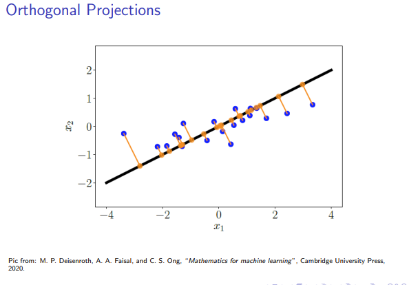
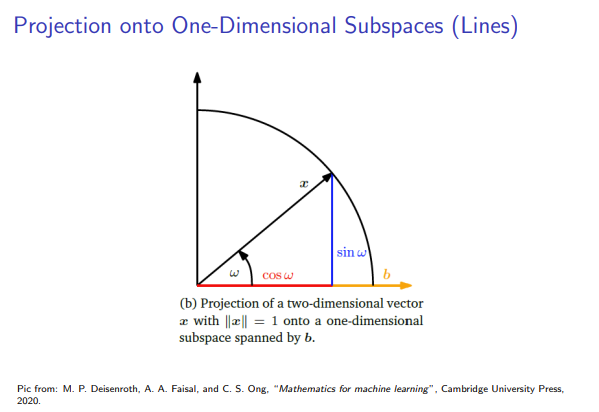
We begin by deriving the projection formula for the simplest case: projecting a vector onto a line. Unless stated otherwise, we assume the standard dot product as the inner product.
- Setup: Let
be a one-dimensional subspace (a line through the origin) spanned by a non-zero basis vector . - Derivation: The projection
must be a scalar multiple of , i.e., . We can solve for the coordinate by using the orthogonality condition . - Final Formulas for 1D Projection:
- Coordinate:
- Projection Vector:
- Projection Matrix:
- Coordinate:
4. Projection onto a General Subspace

The three-step method for 1D projection can be generalized to any m-dimensional subspace
- Setup: Assume we have a basis
for . Construct the basis matrix . - Derivation: The projection
. The orthogonality condition leads to the Normal Equation. - Final Formulas:
- Normal Equation:
- Coordinates:
- Projection Vector:
- Projection Matrix:
- Normal Equation:
Extension: Projections between Subspaces
5. Core Application I: Gram-Schmidt Orthogonalization
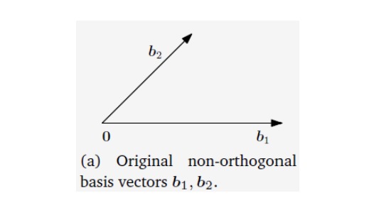
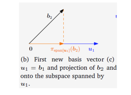
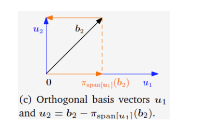
The Gram-Schmidt process is a classic algorithm for constructing an orthonormal basis, and its core idea is the repeated application of orthogonal projection.
-
Goal: To transform a set of linearly independent vectors
into a set of orthogonal vectors that span the same subspace. -
Iterative Construction:
- First Step: Start by choosing the first vector as the beginning of the new basis.
- Subsequent Steps (k=2 to n): For each new vector
, subtract its projection onto the already constructed orthogonal subspace . The remaining component is guaranteed to be orthogonal to that subspace. Since the are already orthogonal, the projection simplifies to:
- First Step: Start by choosing the first vector as the beginning of the new basis.
-
Obtaining an Orthonormal Basis (ONB): After obtaining each orthogonal vector
, simply normalize it. -
Example: Orthogonalize the basis
in . - The resulting orthogonal basis is
.
**拓展:Cholesky分解
6. Core Application II: Projection onto an Affine Subspace
So far, we have discussed projections onto subspaces that pass through the origin. We now generalize this to affine subspaces (e.g., lines or planes that do not pass through the origin).
-
Definition: An affine subspace
can be represented as , where is a support point (a displacement vector) and is a direction subspace parallel to that passes through the origin. -
Solution Strategy: Translate-Project-Translate Back
- Translate to the Origin: Subtract the support point
from both the point to be projected, , and the affine space . This transforms the problem into projecting the new vector onto the familiar direction subspace . - Standard Projection: Compute the orthogonal projection of the vector
onto the subspace , which is . - Translate Back: Translate the result back to its original position by adding the support point
.
- Translate to the Origin: Subtract the support point
-
Final Formula:
-
Mathematical Proof: We want to find the point
that minimizes the distance . - Since
, it can be written as for some . - Minimizing
is equivalent to minimizing . - By definition, the
that minimizes this distance is the projection of onto , so . - Therefore, the closest point is
.
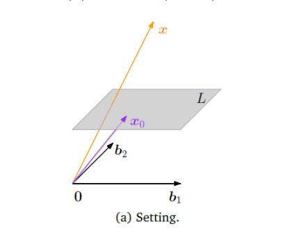
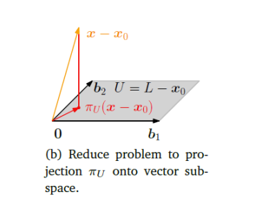
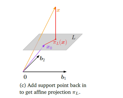
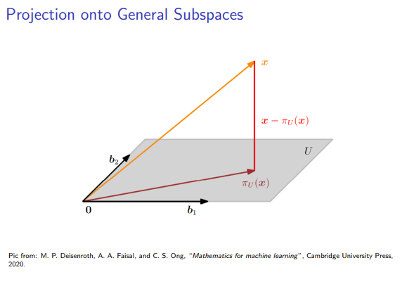
- Since
-
Distance from a Point to an Affine Subspace:
This shows that the distance from a point to an affine space is equal to the distance from the translated point to its corresponding direction subspace.
7. Core Application III: Projections and Least Squares Solutions
Moore Penrose Pseudo inverse
Orthogonal projection provides a powerful geometric framework for solving inconsistent linear systems of the form Ax=b, forming the foundation of the Least Squares Method.
- The Root of the Problem: When the equation
Ax=bhas no solution, it means geometrically that the vectorbdoes not lie within the column space of the matrixA, denotedCol(A). - The Solution Strategy: Since it's impossible to find a point in
Col(A)that is equal tob, we settle for the next best thing: finding the point inCol(A)that is closest tob. - Projection is the Answer: By definition, this "closest point" is precisely the orthogonal projection of
bontoCol(A). We denote this projection as. - Solving the New Equation: We now solve a new system of equations that is guaranteed to have a solution:
The solution to this equation, , is the least-squares solution to the original problem. - Why is it called "Least Squares"? Because this solution
is the one that minimizes the squared length of the error vector, . The squared length of a vector is the sum of the squares of its components, hence the name "least squares."
Part IV: A Detailed Explanation of Rotations
Rotations are another important class of linear transformations, following projections, that play a central role in geometry, computer graphics, and robotics.
1. Fundamental Concepts of Rotation
- Relationship with Orthogonal Transformations: A rotation is a special case of an orthogonal transformation. The core characteristic of orthogonal transformations is that they preserve the length of vectors and the angles between them. Rotations perfectly fit this description.
- Definition: A rotation is a linear function that rotates a plane (or space) by a specific angle
around a fixed origin. - Directional Convention: By convention, a positive angle
corresponds to a counter-clockwise rotation. - Core Property: A rotation only changes the direction of a vector, not its distance from the origin.
2. Rotations in
2.1 Derivation of the
Perspective 1: Basis Change (The "Columns are Transformed Basis Vectors" View)
This is the standard derivation based on the nature of linear transformations.
- Goal: To find a matrix
that, when multiplied by a vector , rotates that vector counter-clockwise by an angle around the origin. - Key Idea: The columns of a linear transformation matrix are the new coordinates of the standard basis vectors after the transformation.
- Derivation Steps:
- Identify Standard Basis Vectors: In
, the standard basis is and . - Rotate the Basis Vectors:
- Rotating
by yields the new coordinates . - Rotating
by yields the new coordinates .
- Rotating
- Construct the Rotation Matrix: Use the transformed basis vectors as the columns of the rotation matrix.
- Identify Standard Basis Vectors: In
Perspective 2: Polar Coordinates and Trigonometric Identities (The "Direct Geometric" View)
This is a more direct geometric proof that does not rely on the idea of basis change.
- Represent the Vector: Express an arbitrary vector in polar coordinates:
. - Represent the Rotation: Rotating this vector by an angle
changes its angle to . The new coordinates are: - Apply Angle-Sum Formulas:
- Write in Matrix Form:
2.2 Applications and Notes for
- Coordinate System Dependency: The derived matrix
only applies directly to vectors expressed in the standard Cartesian coordinate system. - Rotating a Vector in a Non-Standard Basis: If your vector's coordinates
are given in a non-standard basis , the correct procedure is: - Change Basis to Cartesian:
- Rotate with Standard Matrix:
- (Optional) Change Basis Back:
- Change Basis to Cartesian:
- Rotating a Vector Space: To rotate an entire vector space, you simply rotate all of its basis vectors. If the basis of a space is given by the columns of a matrix
, the new rotated basis matrix is .
3. Rotations in
Rotations in 3D are more complex than in 2D because they must occur around an axis of rotation.
- Definition: In
, a rotation is performed around a line (the axis) that passes through the origin. All points on the axis remain fixed during the rotation. - Constructing an Arbitrary 3D Rotation Matrix: A general 3D rotation matrix
can be constructed by determining the new positions of the standard basis vectors after rotation. These new vectors must remain orthonormal.
3.1 Directional Convention for 3D Rotations: The Right-Hand Rule
To define "counter-clockwise," we use the Right-Hand Rule:
- Rule: Point the thumb of your right hand in the positive direction of the axis of rotation. The direction in which your other four fingers curl is the direction of a positive angle (counter-clockwise) rotation.
3.2 Fundamental Rotations about the Coordinate Axes
Any complex 3D rotation can be decomposed into a sequence of fundamental rotations about the three primary axes (x, y, z).
-
Rotation about the x-axis (
) by - Description: The x-coordinate remains unchanged; the rotation occurs in the yz-plane.
- Matrix:
-
Rotation about the y-axis (
) by - Description: The y-coordinate remains unchanged; the rotation occurs in the zx-plane.
- Matrix:
-
Rotation about the z-axis (
) by - Description: The z-coordinate remains unchanged; the rotation occurs in the xy-plane.
- Matrix:
3.3 Trigonometric Proof of the 3D Fundamental Rotation Matrices
- About x-axis: In the yz-plane, let
. After rotating by , the new coordinates are and . Expanding with angle-sum formulas while keeping derives the matrix. - About z-axis: In the xy-plane, let
. After rotating by , the new coordinates are and . Expanding derives the matrix. - About y-axis (Special Case):
- According to the right-hand rule, with the thumb pointing along +y, the fingers curl from the z-axis towards the x-axis.
- Therefore, a rotation from
xtozis considered a negative angle. Alternatively, to achieve a positive rotation, the new angle should be, not . - This explains why the signs of
in the matrix are different from the other two.
3.4 Sequential Rotations in 3D
- Order Matters: In 3D and higher dimensions, rotation is not commutative. That is,
. The order of application is critical. - Matrix Multiplication Order: Rotations are applied sequentially from right to left. If you want to rotate a vector
first about the x-axis, then the y-axis, and finally the z-axis, the combined rotation is calculated as:
4. Rotations in Higher Dimensions (
- Core Idea: Any rotation in n-dimensional space can be described as a rotation within a two-dimensional plane, while leaving the other
dimensions unchanged. - Definition: Givens Rotation
- An n-dimensional rotation matrix that performs a rotation in the
is denoted as . - Its structure is a modified identity matrix. Specifically,
is an 'n x n' matrix, and its form is as follows: - This matrix is an identity matrix everywhere except for four entries, where a standard 2D rotation matrix is embedded:
- An n-dimensional rotation matrix that performs a rotation in the
- Application in Practice:
- In algorithms (like QR decomposition), we typically do not pre-set
. Instead, we back-calculate the values of and to achieve a specific goal, such as zeroing out an entry in a vector.
- In algorithms (like QR decomposition), we typically do not pre-set
5. General Properties of Rotations
- Orthogonality: Rotation matrices
are always orthogonal matrices, satisfying , which means . - Isometry (Distance Preservation):
. Rotations do not change the distance between points. - Angle Preservation: The angle between vectors is unchanged after rotation.
- Commutativity:
- In
, rotations are commutative: . - In
and higher dimensions, rotations are not commutative.
- In